见过这种之后,再读这本书,对一百年前(吗?)的巴黎就有感觉了。海明威说他去新开的咖啡店喝奶油咖啡充饥,我就想到海德堡临河T字路口那家咖啡店了。人来人往的,桌子也不多,但是在这种涌动的拥挤的环境里,那家店竟然能有安静的氛围。不知道会不会贵,所以没去。不过这么个路过瞥了一眼的咖啡店竟然就成了记忆的锚点了。还是应该多记录一些见闻,这几年有很多新鲜的见闻,都空存在语言以及任何媒介之外了。
Where are my memories? Where is my moveable feast?
]]>作者:Léon Bottou, Bernhard Schölkopf
发表: Arxiv
首先我们可以用博尔赫斯的“小径分叉的花园”的隐喻,来类比大语言模型。人们做出一个选择的时候,所付出的代价是放弃了其他所有可能的选择。那如果把所有可能的选择完全考虑进来,就能得到一个充满无数可能性分叉的花园。这个花园,就可以类比“完美语言模型”。它包含了所有可能的人类语言的组合。当它在聊天框输出一串文字的时候,就像是从分叉的小径中选择其中一条一样,或者是人类做出一个选择的时候一样。未被选择的词语构成了其他的分叉。“语言模型”这个全包的概念,是完美的,包含了所有语言的可能性。
实际上,“完美语言模型”就像一本预言书,里面包含了所有我们想要听到的话、可能听到的话。唯一能影响它输出的内容的,就是和它展开对话的那个人。我们用prompt作为引子来引导语言模型的生成,这其实就是对无限的可能性施加限制,prompt完全决定了语言模型的输出。
我们可以先从“幻觉”这个所谓的问题讨论起。其实这不是“幻觉”,而是一种“虚构”,是从人类语言中所有有可能的分叉中,适当地挑选出可能性高的那些,借用了一些合理的逻辑,虚构了另一套合理的故事。“完美的语言模型”,倒不如说是一个“虚构小说机器”。
一类人认为有一些大逆不道的话永远不该存在,所以要求审查LLM;更多的另一类人是希望LLM真的像智能一样为人服务、创造价值,所以要在必要的场合说必要的话。两者为了各自的目的,都希望对LLM这种本身不包含任何是非对错评判偏差的“完美语言模型”进行剪枝,去掉不想要的部分。所用的手段就是用人工精挑细选的语料来微调,或者叫human feedback。
实际上这种审查有很多的问题。最大的问题是,有了“虚构小说机器”之后,它对我们人类文化的影响比想象中大,我们会依赖它来塑造我们的知识和对未来的想象,因此它会影响整个人类的文化。当来到这个层次后,“审查”,或者说“净化”,就变得危险了,因为谁都想把自己的那一套强加在LLM之上,可是谁的标准才是真的标准呢,或者我们真的能有真正的“净化”标准吗?
“在未来,几乎每个人都使用语言模型来丰富他们的思维,对语言模型所写内容的控制权将成为对我们所思考内容的控制权。如此强大的力量能存在而不被滥用吗?
“有些人担心小说机器是一种无所不知的人工智能,可能会比我们活得更久;然而,更黑暗的诱惑是让我们的思想屈服于这个现代的皮提亚,不受真理和意图的影响,但却可以被他人操纵。如果我们一直把小说机器误认为是可以减轻我们思考负担的人工智能,那么语言模型无休止的喋喋不休会让我们像苦苦挣扎的图书馆员一样疯狂。然而,作为小说机器,它们的故事可以丰富我们的生活,帮助我们重温过去,了解现在,甚至瞥见未来。”
作者最后说,人们发明的这种“机器”,不仅能写故事,而且可以写故事的所有变体,这是人类历史上一个重要的里程碑,堪比印刷机的发明。或者,甚至可以比作早在印刷或书写被发明之前的,在洞穴壁画之前就出现的,一种塑造人类的艺术:讲故事的艺术。
]]>references:
https://yang-song.net/blog/2021/score/
https://deeplearning.neuromatch.io/tutorials/W2D4_GenerativeModels/student/W2D4_Tutorial2.html#
https://lilianweng.github.io/posts/2021-07-11-diffusion-models/
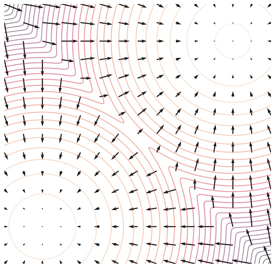 (图中,等高线表示一个概率分布,箭头表示它的分数场。score-based model就是建模这些分数场)
是这样的,前面提到的方法已经讲清楚了神经网络建模和目标函数。但是假如直接拿着数据集(比如图像)让网络学习的话,效果并不好。因为这个score function在低概率密度的区域样本很少,学得也很不好。
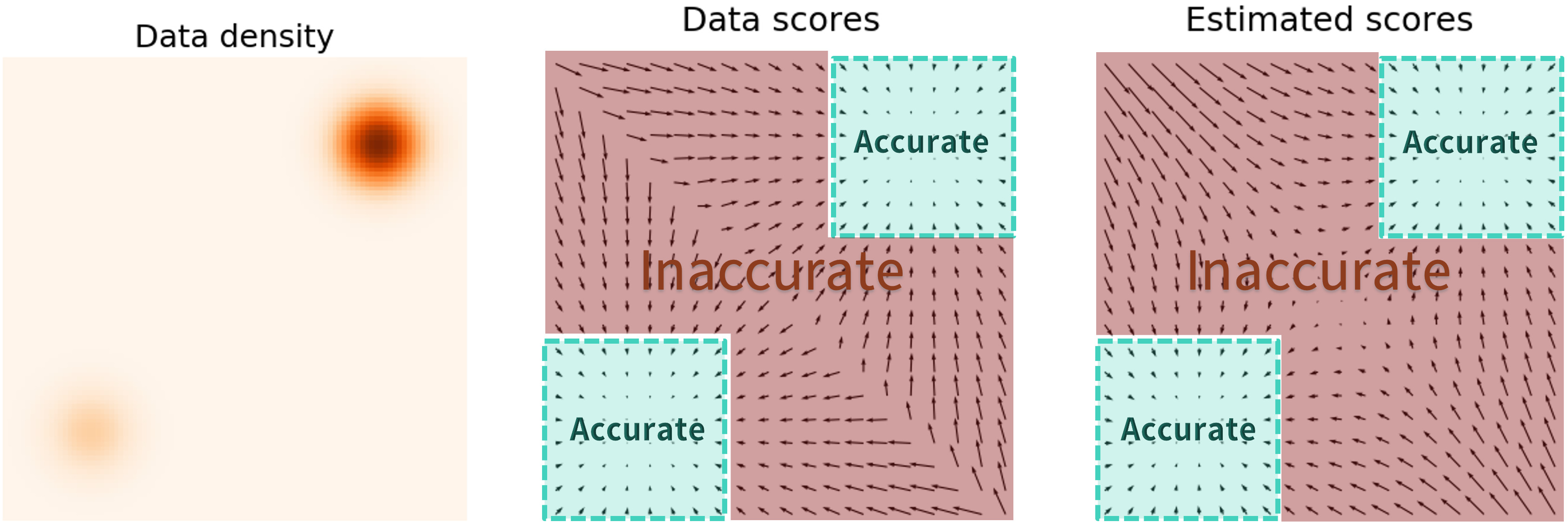
为了解决这个问题,我们才往数据中加 noise,在被噪声扰动后的数据集上训练网络。这些扰动后的数据点极大地扩充了数据集,最主要的是能填充那些低概率密度的分布区域。
大的噪声破坏数据分布,小的噪声不够填充低概率密度区域。所以就用多尺度的噪声。也就是diffusion model的前向过程了。
总体来说,score-based model就是在这些噪声扰动后的数据集上训练的。训练的时候,噪声的尺度当然也可以作为一个已知量输入,也就是noise conditional \(s_\theta(x,i)\)
to read:https://lilianweng.github.io/posts/2021-07-11-diffusion-models/
从diffusion models的角度解释整个模型
]]>作者:Hsuan-I Ho, Lixin Xue, Jie Song, Otmar Hilliges。ETH
发表: CVPR23
链接: https://custom-humans.github.io/
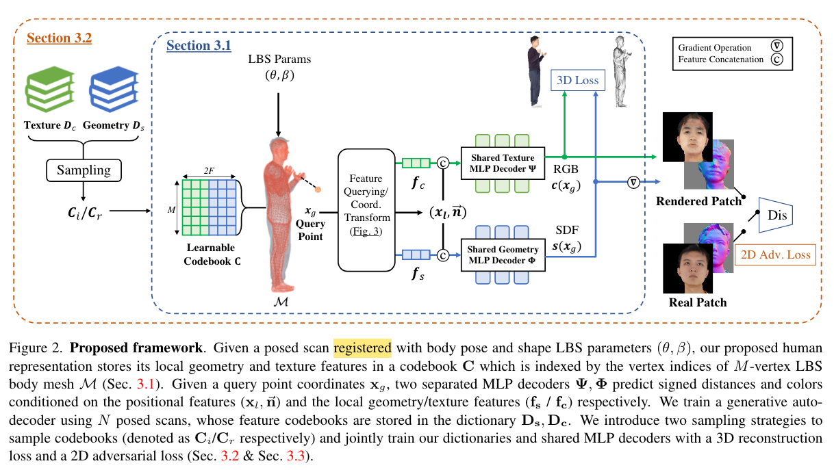
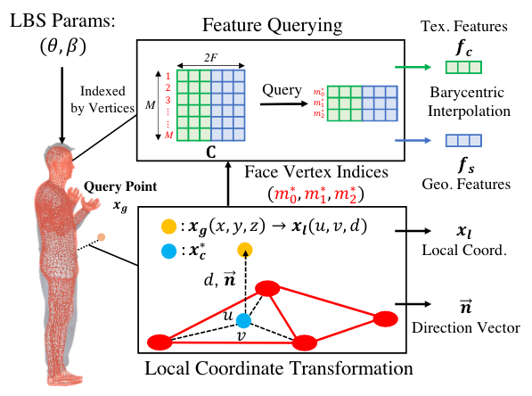
混合的3D人体representation:
有一个可学习的特征codebook,包含\(M\times 2F\)个特征,其中\(F\)个是几何特征,另外\(F\)个是外貌特征。给定一个human mesh,mesh有M个顶点(M很大,一万多),每个顶点跟codebook中的特征显式地一一对应。
当NeRF渲染时,给定空间中一个query点,提取局部的特征:
采样个体样本时,有两种方式:
训练过程
一些编辑方式
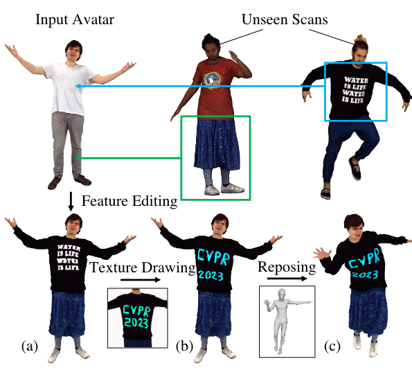
初始化:采样一个3D数字人样本。也就是前面提到的两种采样方式,可以采样已有的,也可以采样全新生成的
optimize特征,拟合一个3D扫描人体。用到的是3D loss
跨个体的特征编辑:简单粗暴,先用Blender选择人体局部对应的顶点,然后把想要的样本的codebook中的那部分特征交换到目标的codebook来
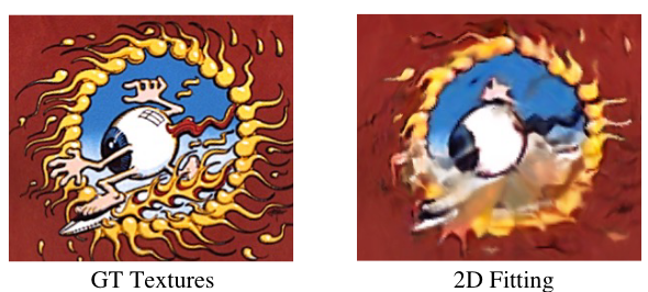
绘制材质:拿到渲染后的2D图像后,可以直接对2D图像进行一些绘制,然后再用它监督训练codebook。后面的实验结果看上去效果还不错,但limitation说不能很好地拟合过于高精度的细节
更换人体姿势:这个representation本身是由一个SMPL mesh加一个codebook组成的;只要对SMPL mesh的参数进行修改,就能直接改变姿势了
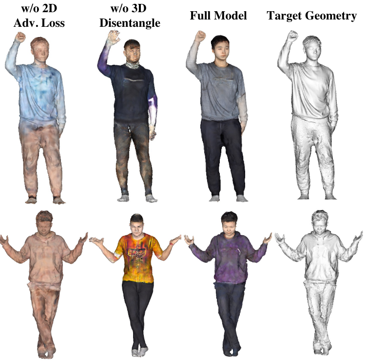
实验
作者:Gusi Te, Xiu Li, Xiao Li, Jinglu Wang, Wei Hu, and Yan Lu
发表: ECCV 2022
链接: https://arxiv.org/abs/2208.08728
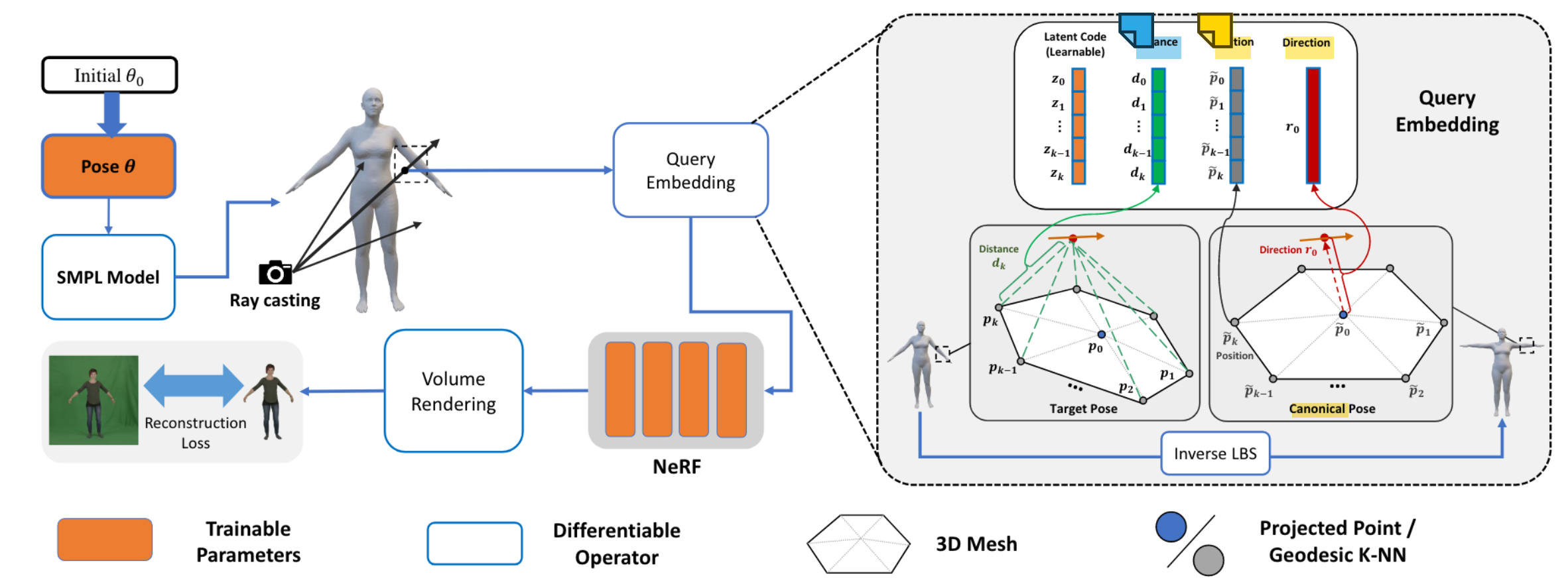
精髓就在图里了:
人体的表现形式是我们熟悉的:首先有一个由pose参数\(\theta\)驱动的SMPL mesh,以及一个mesh-guided NeRF,后者的输入是对应query ray上的3D points的embedding
Query embedding的具体构成:
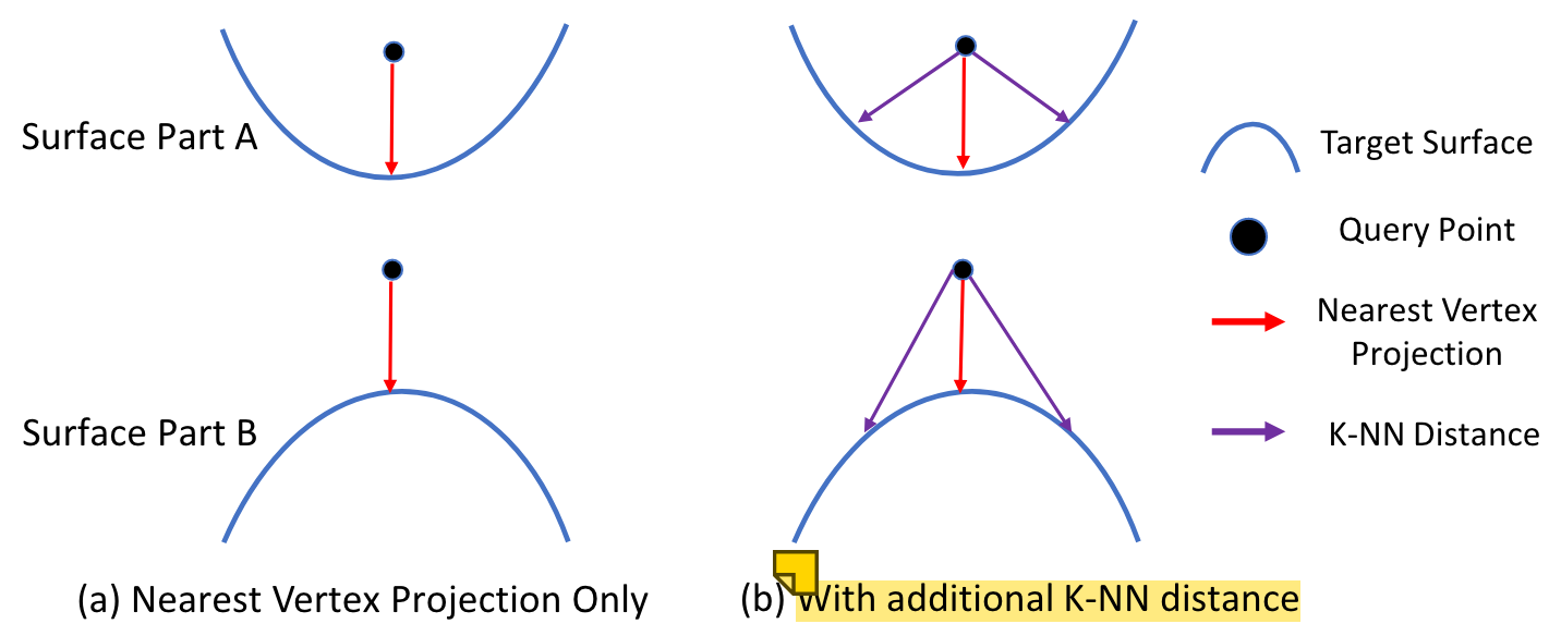
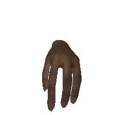
文中特意用上图强调了这里需要用到K近邻顶点,而不是单个最近的顶点。因为如果只用单个最近的顶点(图a),就不能提供不同的deformation pattern 的信息;而(b)里加上了K-NN distance之后,就能有这个deformation pattern信息了。(我有点疑惑什么是deformation pattern,就是这个表面的凹凸性吗?)
References:
https://zhuanlan.zhihu.com/p/45131536
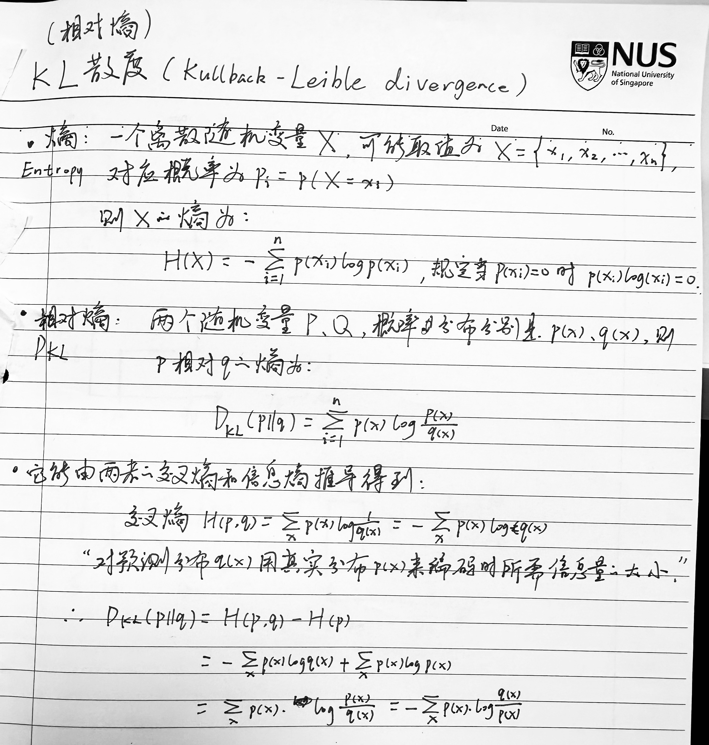
https://hsinjhao.github.io/2019/05/22/KL-DivergenceIntroduction/
https://www.jiqizhixin.com/articles/2018-05-29-2
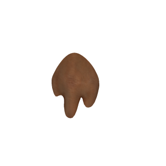
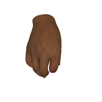
作者:Rolandos Alexandros Potamias, Stylianos Ploumpis, Stylianos Moschoglou, Vasileios Triantafyllou, Stefanos Zafeiriou. From Imperial College London and Cosmos.
发表: CVPR23
链接: https://github.com/rolpotamias/handy

如果你去做这个任务,会怎么做?作者做的方法和你想的有什么差异?
Q:我感觉这个任务听起来还挺直观的,就是用GAN去训练外观,定义一些更多vertices的mesh template,用超级大量的样本去训练堆效果嘛?hand model的定义会有什么新意吗?我倒是想不出来。
A:确实很直观,hand model的定义没什么太大区别。贡献点主要在于:1. 很大很好很variant的新数据集,造成了很好的Handy 2. 用StyleGAN来学texture,而不是传统的PCA,得到的texture更高频细节,更好。
读前疑问:
raw scan:3000 vertices meshes。1208个人,包括关于他们的meta data,比如性别,年龄,身高,种族等。这些人的diversity比较大
(Useful) egoist / openai-proxy
用 Vercel 开一个小的 Proxy server,转发 gpt API,这样可以绕开有些国家地区的 IP 限制
BuilderIO / ai-shell
在命令行里使用 chatgpt,把自然语言转化成 Linux commands,命令是 ai [texts]
eli64s / readme-ai
一个轻量的 script,根据 repository 生成酷炫的 readme 文件
efJerryYang / chatgpt-cli
命令行 chatgpt client
yufeikang / ai-cli
另一个命令行 chatgpt client(实测的时候再对比一下这俩)
mukulpatnaik / researchgpt
输入论文 PDF 文件,然后和 gpt 聊论文。一个用 Flask 开发的 web client 貌似,可以再仔细看一下咋实现的,挺有意思
(⭐️ Amazing) AntonOsika / gpt-engineer
很方便安装,pip install 就好了!直接通过描述 + AI 追问 + 补充细节,生成一个代码项目
(⭐️ Amazing) Yidadaa / ChatGPT-Next-Web
好像很实用的 web GUI!一键部署到 Vercel。我找这玩意主要是为了直接用 API 访问 GPT-4,就不用订阅每个月的 ChatGPT Plus 了,后者太贵了,也用不了那么多

回国,这个词对我来说不算什么,身处国内的时候,自己是没有概念的。只有在国外的时候,才对国内有概念。这一点真是讽刺。国内的时间匆匆而过,以前会为了在国外多待几年而争取,争取到了又雀跃。现在真要待那么多年了,才感到自己正坐在什么飞驰而远去的列车上。
人生在世,奔头这个词,我是想解构它的。人活着不为了什么,活就活了。可是我分明在努力什么,在抓住些什么。嘴硬罢了,谁能超凡脱俗,没点惦念的东西?亲人,向往的某种生活,成就感,这就是我的奔头。只是:停在原地原来是一种幸运,也是一种特权。
]]>我最痛恨别人,半熟不熟的人见面,跟你打招呼,问你家里近况怎么样。我很生气,简直想骂回去。可是你骂了吧,人家觉得你是神经病。可是我要怎么回答呢?我这两个儿子,一个工作都丢了,一个身体又那样不好。
我命苦啊。我从小家里穷,也没人管我。13岁就出去工作养活自己了。跟了你爷爷,过的都是苦日子。他一个月三十四块五角钱,二十块钱给他爸妈,雷打不动的。家里饭都吃不起了,也要给。剩下十四块五,十块钱给我,他留四块五。抽最差的烟,走得那么早。
我要管家里所有事。他什么也不管啊,一日三餐,他妈,两个儿子,去河边洗衣服。我还要上班。我每天都好累。
好不容易,日子稍微好一点了。他又走了!我那时简直恨他。
别看我现在这样,现在是我最轻松的日子。共产党给我发钱。所以我说,感谢共产党。我拿自己的钱,过自己的日子!就是记性不好。人活到连自理能力也没有了,还有什么意思。跟你爸说好了,到时候我死在这间屋子了,就火化。我都看得开。
死!我听到就眼泪直湍湍地流。奶奶说,不说这个了。她也抹眼泪。
奶奶一个月领三千多退休工资,自己省吃俭用,只花得了一千多。剩的,存在那,每年寒暑假我和妹妹去看她,她发给我们。
我说爸爸,你帮我把钱退给她。
爸爸说你拿着。她自己花不完,这钱不给你们,她拿着有什么用了?给了她安心。
我走的时候,她送出屋子,送到楼梯口。
我走远了,爸爸说,你回头再给奶奶挥挥手,你看她在阳台上看你呢。
我转头看到一簇花白的头发,远远的,很小。
能不能不要有离别呢?
]]>有哪些?
这里的坑在于,camera本身支持任意坐标系,比如Freihand提供的是screen是224*224的相机坐标系。但是,render是默认NDC坐标系的!也就是normalized coordinate system,x和y是normalized到[-1,1]的。
一开始我直接把相机内参传给PerspectiveCameras,并且定义我的相机screen是224*224,像这样:
1 | cameras = PerspectiveCameras(K=ks, image_size=((224,224),)) |
完全不报错,就是有问题:render 过后没东西在画面上。
我最后在官方文档找到不起眼的一句:
The PyTorch3D renderer for both meshes and point clouds assumes that the camera transformed points, meaning the points passed as input to the rasterizer, are in PyTorch3D's NDC space.

我一看,原来默认PerspectiveCameras是ndc坐标系的,in_ndc = False by default!
所以解决方法就是:
Screen space camera parameters are common and for that case the user needs to set
in_ndctoFalseand also provide theimage_size=(height, width)of the screen, aka the image.
那么加一个参数就好了,可是谁知道这问题困扰了我整整两三天:
1 | cameras = PerspectiveCameras(K=ks, in_ndc=False, image_size=((224,224),)) |
另外,我还找到了如下这个等价方法,是先把内参转到NDC坐标系,再传给PerspectiveCameras。(至于为什么探索到这个方法,在后面问题 3 里可以找到原因…)
1 | def get_ndc_fcl_prp(Ks): |
注意focal_length=-fcl,这个负号是为什么呢?这是另一个坑了哈哈哈哈。
答案是:pytorch3d坐标系的convention和我的相机不一样,它是+X指向左,+Y指向上,+Z指向图像平面外。这其中有个上下左右镜像的关系。
cv2的图像是BGR(老生常谈了),pytorch3d的是RGB。如果图像的黄蓝色相反了,基本就是这个问题,需要翻转一下,可以用torch的clip(dim=(2,))
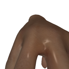
锯齿就是说像下图这样,物体的边缘很尖锐,像素点粒粒分明!
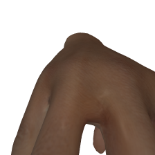
下面是我抗锯齿处理后的效果,可以看见边缘柔和了很多:

(我真的搞了一周这个问题……看看我的心路历程:
blur_radius 和 faces_per_pixel 应该调大一些?这其实是一个很直观的想法了,甚至一个有经验的学长看了之后都告诉我应该是这个问题。可是当我疯狂调大这两个参数,发现并没有改变这个问题。blur_radius 只会让物体内部的材质更模糊,但是边缘的锯齿完全没改变。faces_per_pixel更是无益,几乎不影响效果。1024x1024,发现锯齿边缘的确是不明显了!可是我又看了相机拍摄的原始图像,虽然是有点模糊,但是不至于这么大的锯齿呀,肯定还有别的问题。)终于,在这个issue里找到同样的问题:https://github.com/facebookresearch/pytorch3d/issues/399
解决方案是:
render at a higher resolution and then use average pooling to reduce back to the target resolution
居然这么暴力……不过issue里面有很详细的解释,也能理解,这就是render原理之外需要考虑的事情,甚至算不上什么bug。
代码如下:
1 | import torch.nn.functional as F |
一开始,皮肤 render 出来像这样,跟陶瓷似的,像话吗:
改进后,效果这样,自然多了:
其实搞清楚材质相关的一些参数就好了。主要来说,这个反光是由这两个量决定的:
specular_color: specular reflectivity of the material,指定镜面反射颜色,在表面有光泽和镜面般的地方看到的颜色。shininess:定义材质中镜面反射高光的焦点。 值通常介于 0 到 1000 之间,较高的值会产生紧密、集中的高光。注意这里是改物体material的这些参数。虽然lighting也有这些参数定义,但这是关于光源的,和这个反光没有关系。
所以修改很简单:定义materials类,调整specular_color。默认是1,1,1,就是纯白色;调成0.2,0.2,0.2比较适合人的皮肤。
1 | from pytorch3d.renderer import Materials |
还是一只手的模型,render 出来居然只有半个手背,距离相机更远的部分像是被截断了:
改进后,正常的效果应该是这样才对:
所以问题出在哪呢?的确是“更远的部分被截掉了”。我找到了RasterizationSettings里有这么一个相关的参数:
可是问题不在这个参数上,因为它的默认值就是None,应该在后续都没有影响。
经过仔细看源码,我发现问题出在SoftPhongShader……具体来说,在shader.py 第138-139行,SoftPhongShader的forward函数里:
1 | znear = kwargs.get("znear", getattr(cameras, "znear", 1.0)) |
居然有一个默认的z范围[1,100]……………………所以其实是我的mesh的scale太大了,再加上相机的dist比较大,整个深度就超过zfar了。所以有两种方法,要么缩小一下mesh的尺度;要么不想改变原数据的话,在render的时候,把znear zfar参数额外传入,如下:
1 | images = renderer(mesh, ..., znear=-2.0, zfar=1000.0) |
我的数据中3D mesh的材质用了PBR(physical based rendering)。它提供三张贴图图像:diffuse map,specular map和normal map。
但是pytorch3d目前并不支持PBR inspired shading(see issue)。
所以目前我只能把diffuse map作为一般意义上的texture map,而忽略了specular map和normal map这两张图。
我不确定能不能自己实现这部分功能,比如自定义 phong_shading函数(参考issue)。但这有点超出我的能力范围和精力范围,所以暂时搁置了。如果能实现的话,PyTorch3D 似乎是欢迎contribution的(issue)
In general, the camera projection matrix P has 11 degrees of freedom: \[P=K[R\ \ \ t]\]
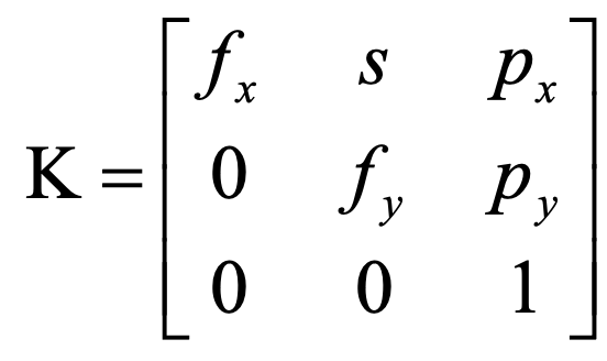
| Component | # DOF | Elements | Known As |
|---|---|---|---|
| K | 5 | \(f_x, f_y, s,p_x, p_y\) | Intrinsic Parameters; camera calibration matrix |
| R | 3 | \(\alpha,\beta,\gamma\) | Extrinsic Parameters |
| t (or \(\tilde{C}\)) | 3 | \((t_x,t_y,t_z)\) | Extrinsic Parameters |
3D world frame ----- R, t ----> 3D camera frame ------ K -----> 2D image
Explanation:
P: Projective camera, maps 3D world points to 2D image points.
K: Camera calibration matrix, 3 x 3, \(x=K[I|0]X_{cam}\), given 3D points in camera coordinate frame \(X_{cam}\), we can project it into 2D points on image \(x\).
R and t: Camera Rotation and Translation, rigid transformation. \(X_{cam}=( X,Y,Z,1)^T\) is expressed in the camera coordinate frame. In general, 3D points are expressed in a different Euclidean coordinate frame, known as the world coordinate frame. The two frames are related via a rigid transformation (R, t).
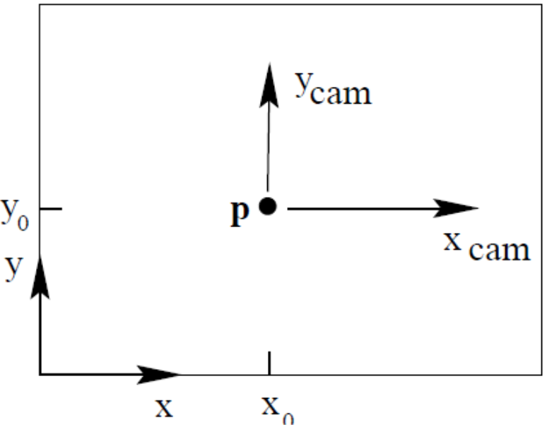
P: 3x4, homogeneous, camera projection matrix, \(P=diag(f,f,1)[I|0]\). P is K without considering \((x_{cam},y_{cam})\) in the image. (In other words, it simplify \((p_x, p_y)=(0,0)\).
[username].github.io, I have a domain jyzhu.top, and want to use my custom domain.Rename the blog repo as blog; rename the academic page repo as [username].github.io.
Edit the blog's Hexo config file:
1 | url: https://jyzhu.top/blog |
While no need to move all the files into a subfolder blog of your repo.
The Jekyll config is simple. Nothing needs to specify.
Edit the Github repo settings. Set the academic repo's custom domain as jyzhu.top. A CNAME file will be automatically added in the root. Now obviously, the jyzhu.top successfully refers to the academic page.
Then you know what, everything is done! Because all other repos with github page turns on, are automatically mapped to subpaths of [username].github.io by Github. Then coz [username].github.io is mapped to [url], everything will be there, including [url]/blog for the blog repo.
The hexo-douban plugin cannot render styles now. Need to fix.
Update:
loading.gif in the index.js of this pluginthen it seems ok now.
]]>之前不理解为什么要用一个和从小到大学的笛卡尔坐标系不同的齐次坐标系来表示东西,并且弄得很复杂;学了各种公式也很糊涂。现在终于明白了
就是用来表示现实世界中我们眼睛看到的样子:两条平行线在无限远处能相交。
就是用N+1维来代表N维坐标。
也就是说,原本二维空间的点\((X,Y)\),增加一个维度,用\((x,y,w)\)来表示。把齐次坐标转换成笛卡尔坐标是很简单的,对前两个维度分别除以最后一个维度的值,就好了,即 \[X=\frac x w,\ Y=\frac y w\\ (X,Y)=(\frac x w,\frac y w)\]
这样做就可以表示两条平行线在远处能相交了!why?
要解释这个,需要先解释一个齐次坐标系的特点:规模不变性(也是叫homogeneous这个名字的原因)。也就是说,对任意非零的k,\((x,y,w)\)和\((kx,ky,kw)\)都表示二维空间中同一个点\((\frac x w,\frac y w)\)。(因为\(\frac{kx}{kw}=\frac xw\)嘛。)
首先,用原本笛卡尔坐标系中的表示方法,无限远处的点会被表示成\((\infty,\infty)\),从而失去意义。但是我们发现用齐次坐标,我们就有了一个方法明确表示无限远处的任意点,即,\((x,y,0)\)。(为什么?因为把它转换回笛卡尔坐标,会得到\((\frac x 0,\frac y 0)=(\infty,\infty)\))。
现在,用初中所学,联立两条直线的方程,得到的解是两条直线的交点。假如有两条平行线\(Ax+By+C=0\)和\(Ax+By+D=0\),求交点,则 \[\left\{\matrix{Ax+By+C=0 \\Ax+By+D=0}\right.\] 在笛卡尔坐标系中,可知唯一解是\(C=D\),即两条线为同一条直线。
但是,如果把它换成齐次坐标,得到 \[\left\{\matrix{A\frac x w+B\frac y w+C=0\\ A\frac x w + B\frac y w +D=0}\right.\]
\[\left\{\matrix{Ax+By+Cw=0\\Ax+By+Dw=0}\right.\]
当\(w=0\),上式变成\(Ax+By=0\),得到解\((x,-\frac {A}Bx,0)\)。其实这里的x和y是什么不重要,重要的是w=0,意味着这是个无限远处的点。也就是说,两条平行线在无限远处相交了!甚至能明确求出交点!
]]>Reference:
http://www.songho.ca/math/homogeneous/homogeneous.html
https://zhuanlan.zhihu.com/p/373969867
Reference: Original NeRF paper; an online ariticle
在已知视角下对场景进行一系列的捕获 (包括拍摄到的图像,以及每张图像对应的内外参),合成新视角下的图像。
NeRF 想做这样一件事,不需要中间三维重建的过程,仅根据位姿内参和图像,直接合成新视角下的图像。为此 NeRF 引入了辐射场的概念,这在图形学中是非常重要的概念,在此我们给出渲染方程的定义:
那么辐射和颜色是什么关系呢?简单讲就是,光就是电磁辐射,或者说是振荡的电磁场,光又有波长和频率,\(波长\times 频率=光速\),光的颜色是由频率决定的,大多数光是不可见的,人眼可见的光谱称为可见光谱,对应的频率就是我们认为的颜色:
How is this implemented?
The MLP is designed to be two-stages:
For each pixel, sample points along the camera ray through this pixel;
For each sampling point, compute local color and density;
Use volume rendering, an integral along the camera ray through pixels is used: \[C(\bold r)=\int_{t_1}^{t_2} T(t)\cdot \sigma (\bold r(t))\cdot \bold c(\bold r(t),\bold d)\cdot dt \\T(t)=\exp (-\int_{t_1}^t \sigma(\bold r(u))\cdot du)\] We can get the color C of the pixel.
This can be implemented by sampling approaches.
Now everything can be approximated: \[\hat C(\bold r)=\sum_{i=1}^N \alpha_iT_i\bold c_i \\T_i=\exp (-\sum_{j=1}^{i-1}\sigma_i\delta_j) \\\alpha_i=1-\exp(\sigma_i\delta_i)\\\delta_i=\text{distance between sampling point i and i+1}\]
\[L=\sum_{r\in R}\| \hat C(\bold r)-C_{gt}(\bold r)\|^2_2\]
Similar to the above formulas, expected depth can also be calculated, and can be used to regularize the depth smoothness.
It is required to greatly improve the fine detail results.
There are many other positional encoding techs, including trainable parametric, integral, and hierarchical variants
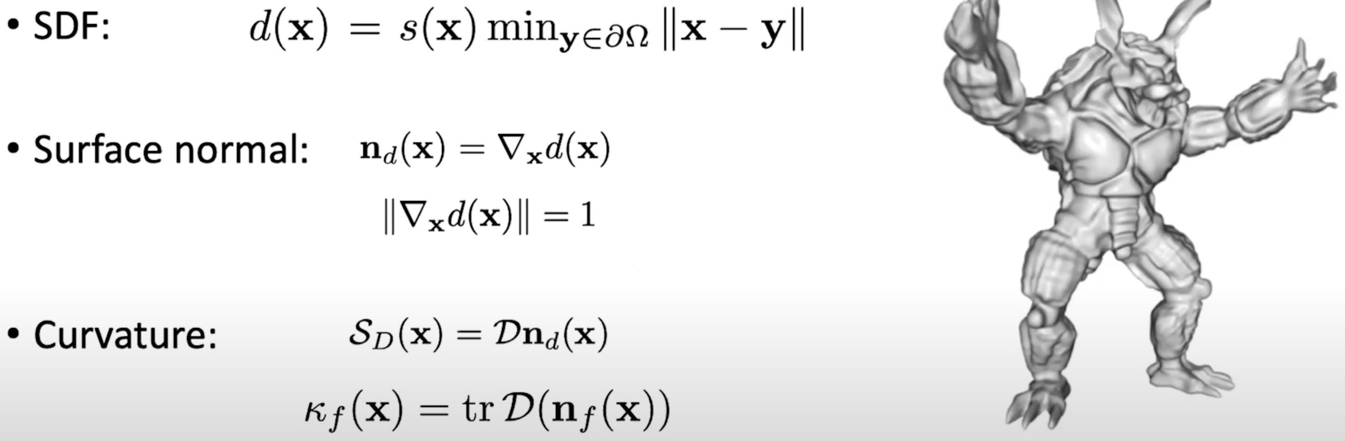
SDF是一种计算图形学中定义距离的函数。SDF定义了空间中的点到隐式曲面的距离,该点在曲面内外决定了其SDF的正负性。
相较于其他像点云(point cloud)、体素(voxel)、面云(mesh)那样的经典3D模型表示方法,SDF有固定的数学方程,更关注物体的表面信息,具有可控的计算成本。
\[\arg \min_x\|y-F(x)\|+\lambda P(x)\]
y is multiview images, F is forward mapping, x is the desired 3D reconstruction.
F can be differentiable, then you can supervise this.
This is part of my journey of learning NeRF.
Mildenhall et al. introduced NeRF at ECCV 2020 in the now seminal Neural Radiance Field paper.
This is done by storing the density and radiance in a neural volumetric scene representation using MLPs and then rendering the volume to create new images.
GIRAFFE: Compositional Generative Neural Feature Fields
2021年CVPR还有许多相关的精彩工作发表。例如,提升网络的泛化性:
针对动态场景的NeRF:
其他创新点:
Zero-Shot Text-Guided Object Generation with Dream Fields
NeRF at NeurIPS 2022 - Mark Boss
Bigger to learn:
Neural fields is ready to be a prime representation, similar as point clouds or meshes, that is able to be manipulated.
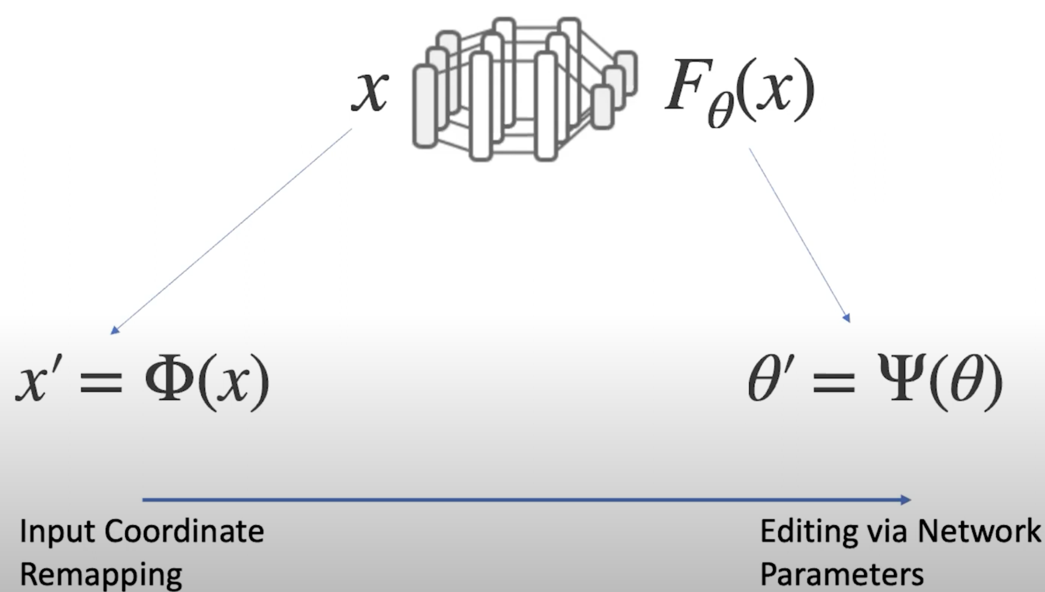
You can either edit the input coordinates, or edit the parameters \(\theta\).
On the other axis, you can edit through an explicit geometry, or an implicit neural fields.
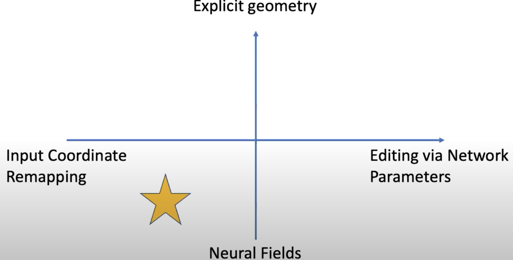
The following examples 落在不同的象限。
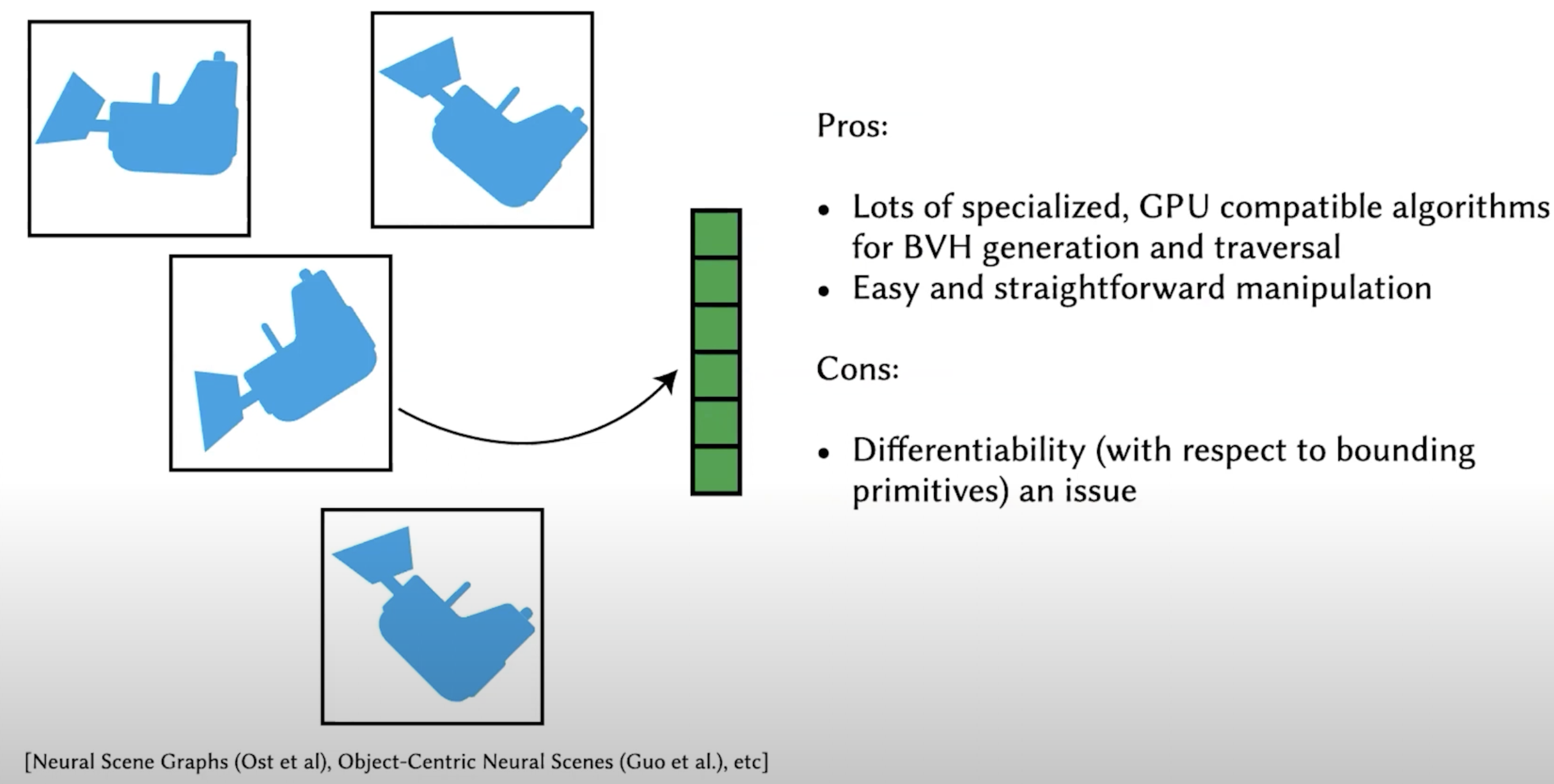
You can represent each object using a separated neural field (local frame), and then compose them together in different ways.
If you want to manipulate not only spatially, but also temporaly, it is also possible. You can add a time coordinate as the input of the neural field network, and transform the time input.
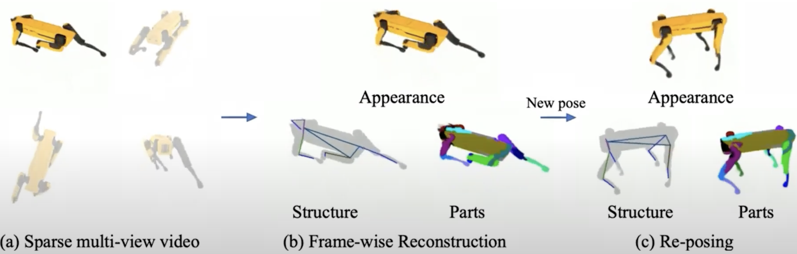
You can also manipulate (especially human body) via skeleton.
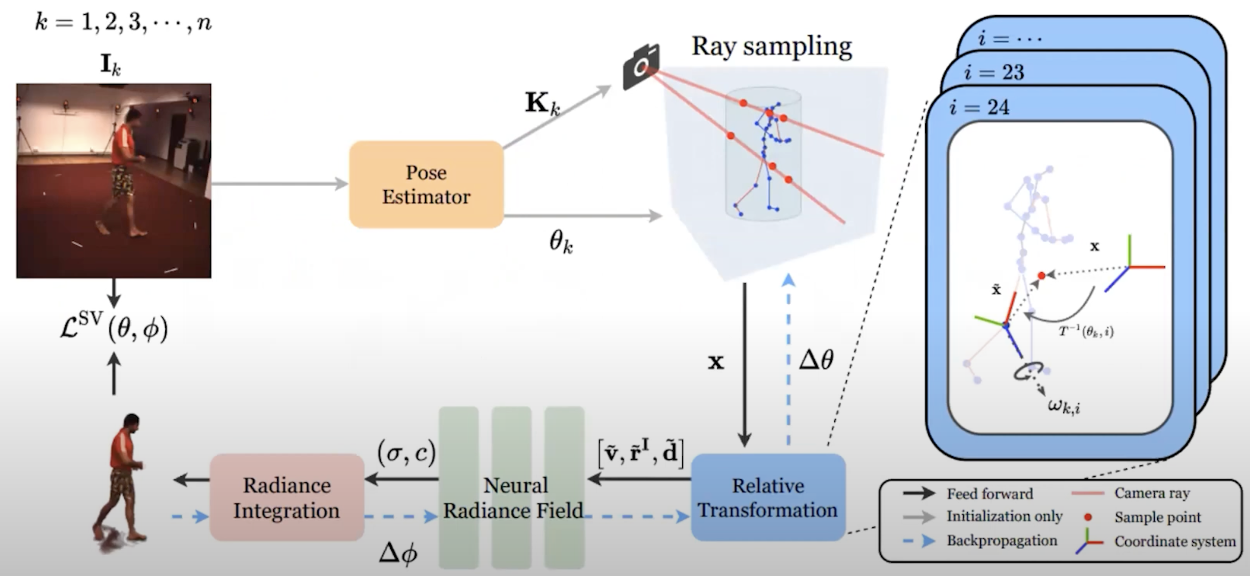
Beyond human, we can also first estimate different moving parts of an object, to form some skeleton structure, and then do the same.
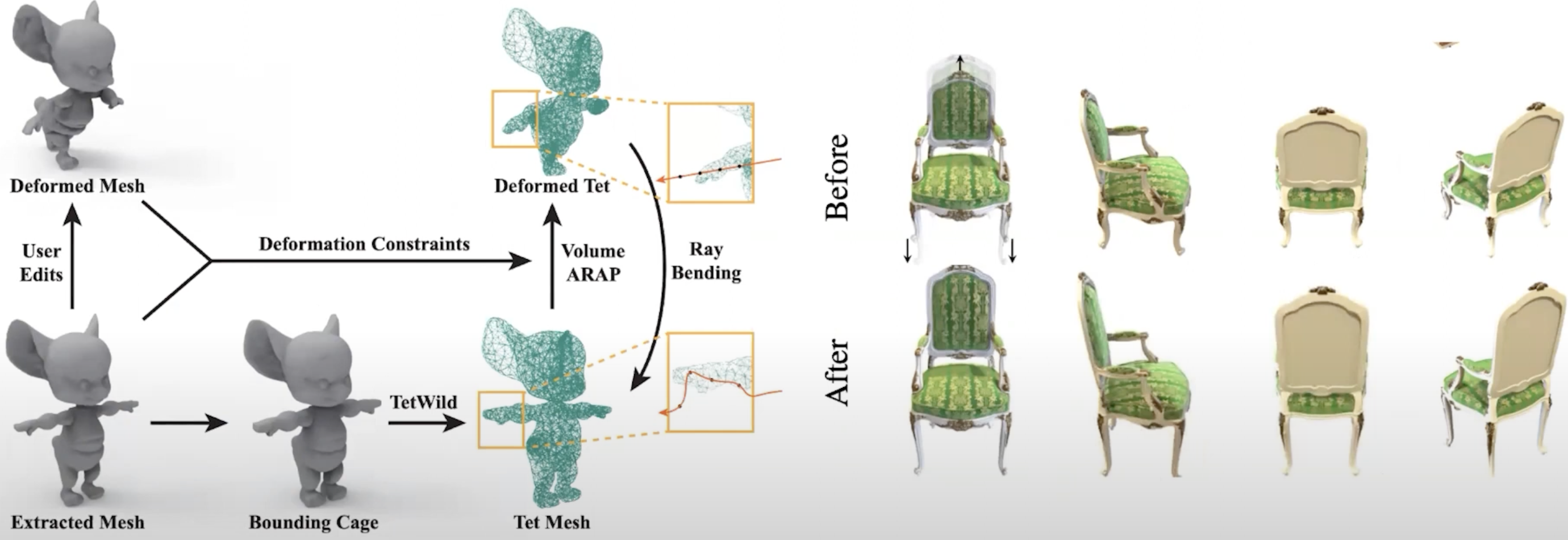
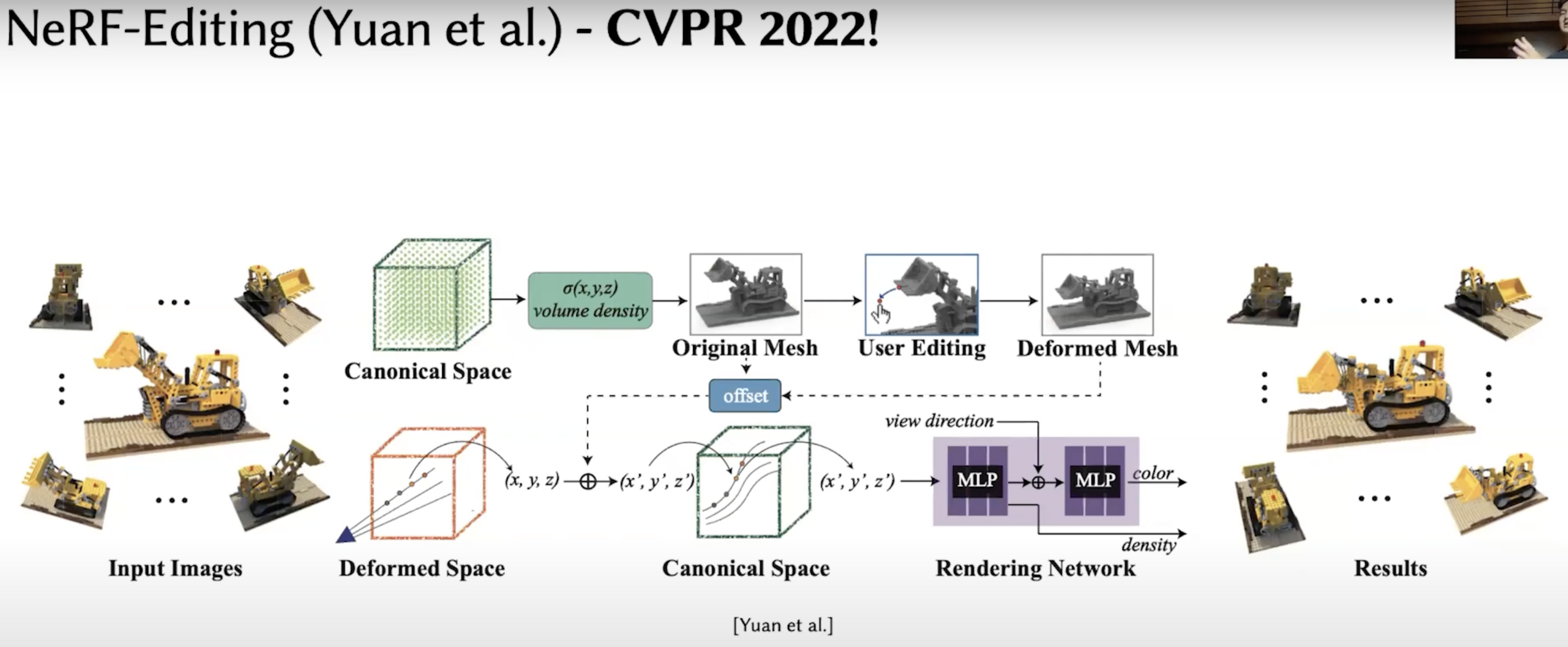
Beyond rigid, we can also manipulate via mesh. coz we have plenty of manipulation tools on mesh. The deformation on mesh can be re-mapped as the deformation on the input coordinate
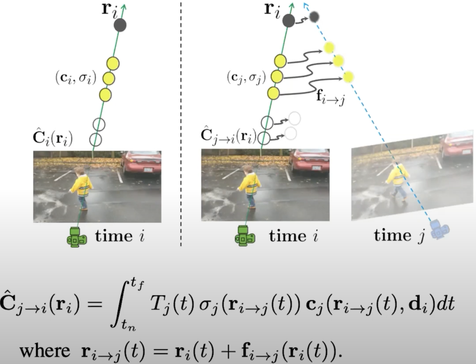
We use the \(f_{i\rightarrow j}\) to edit the \(r_{i\rightarrow j}\) to represent one ray into another one.
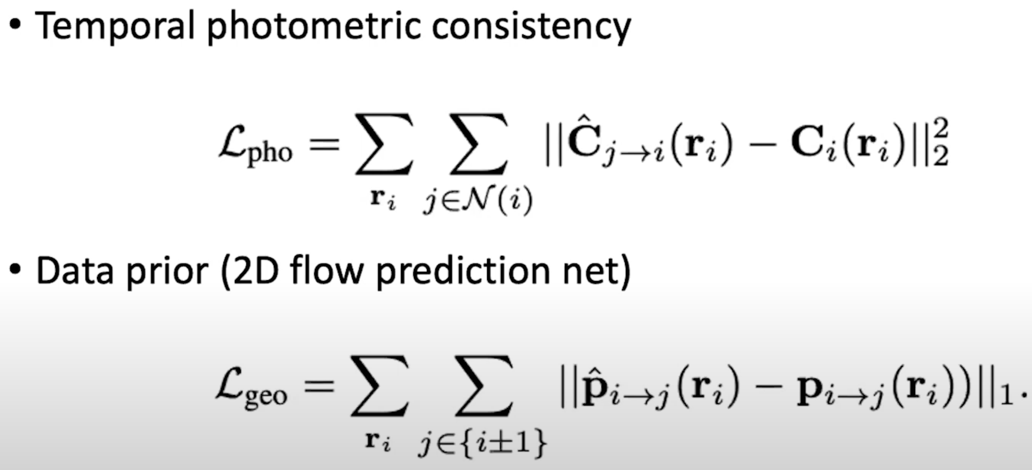
We need to define the consistency here, so that the network can learn through forward and backward:
The knowledge is already in the network. So instead of editing the inputs, we can directly edit the network parameters for generating new things.

It decomposes the network into shape and color networks, and we can edit each independently.

Volume rendering can render fogs. Sphere rendering only render the solid surface, and needs ground truth supervision.? Neural renderer combines the two.
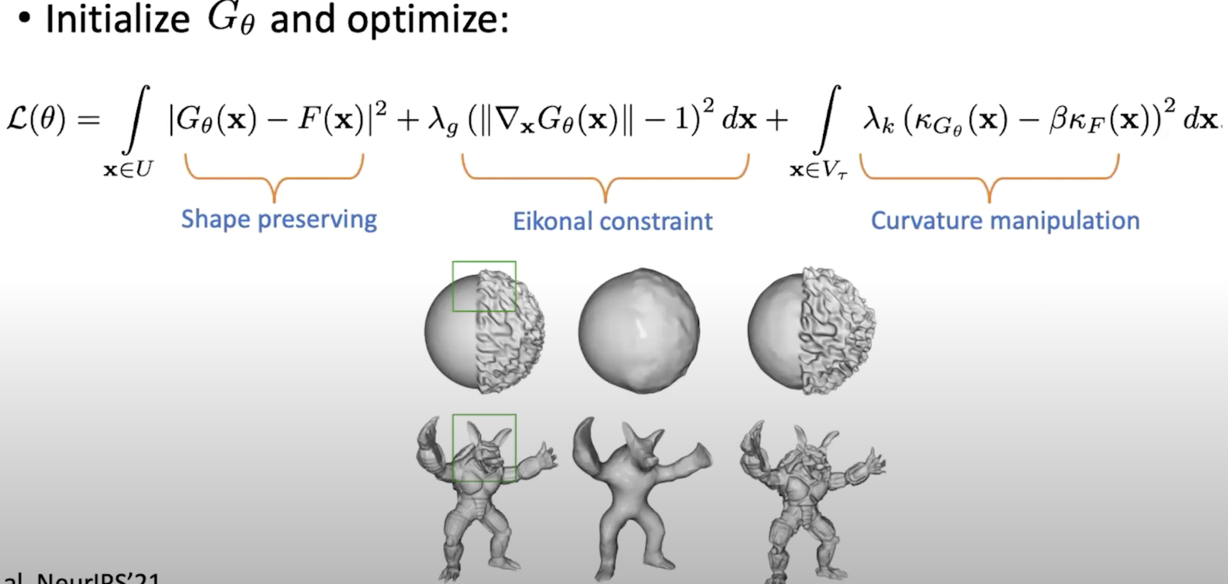
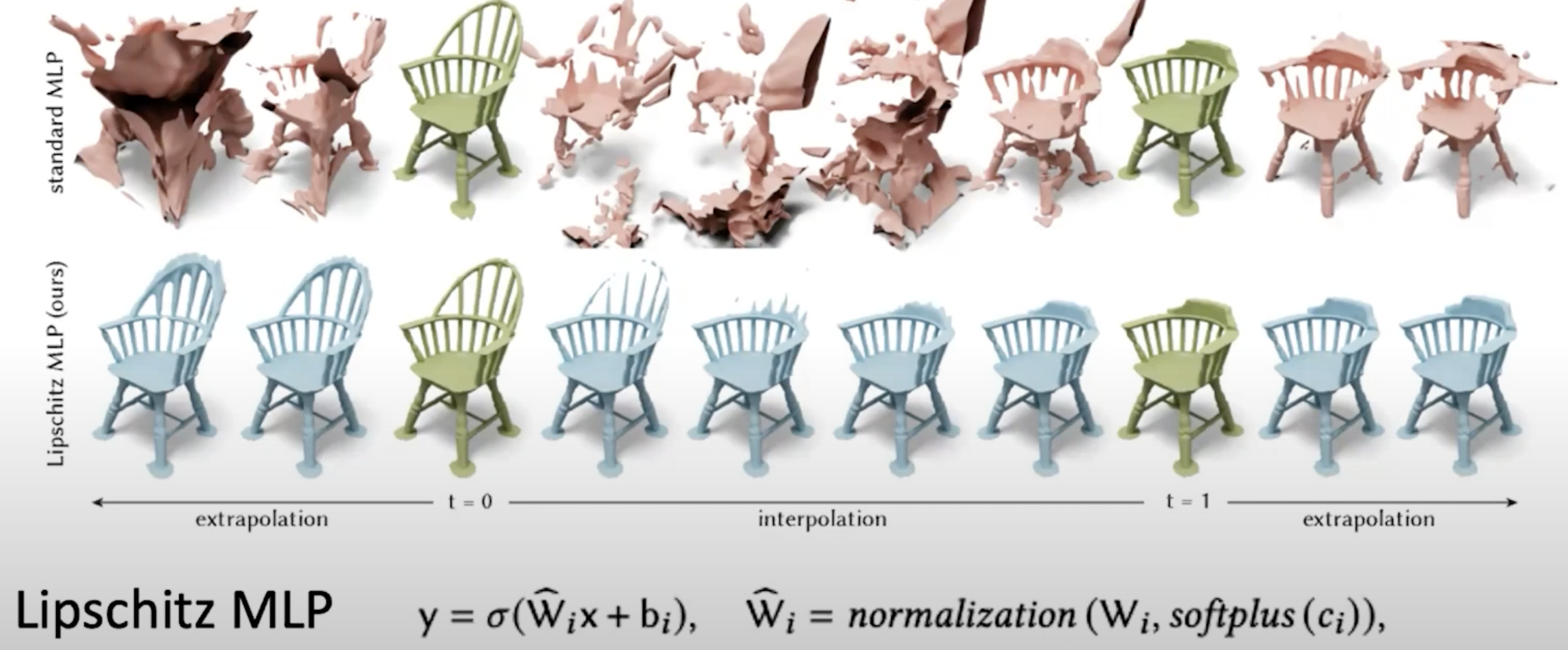
Design a neural network with higher order derivatives constraints and therefore directly use its derivative.
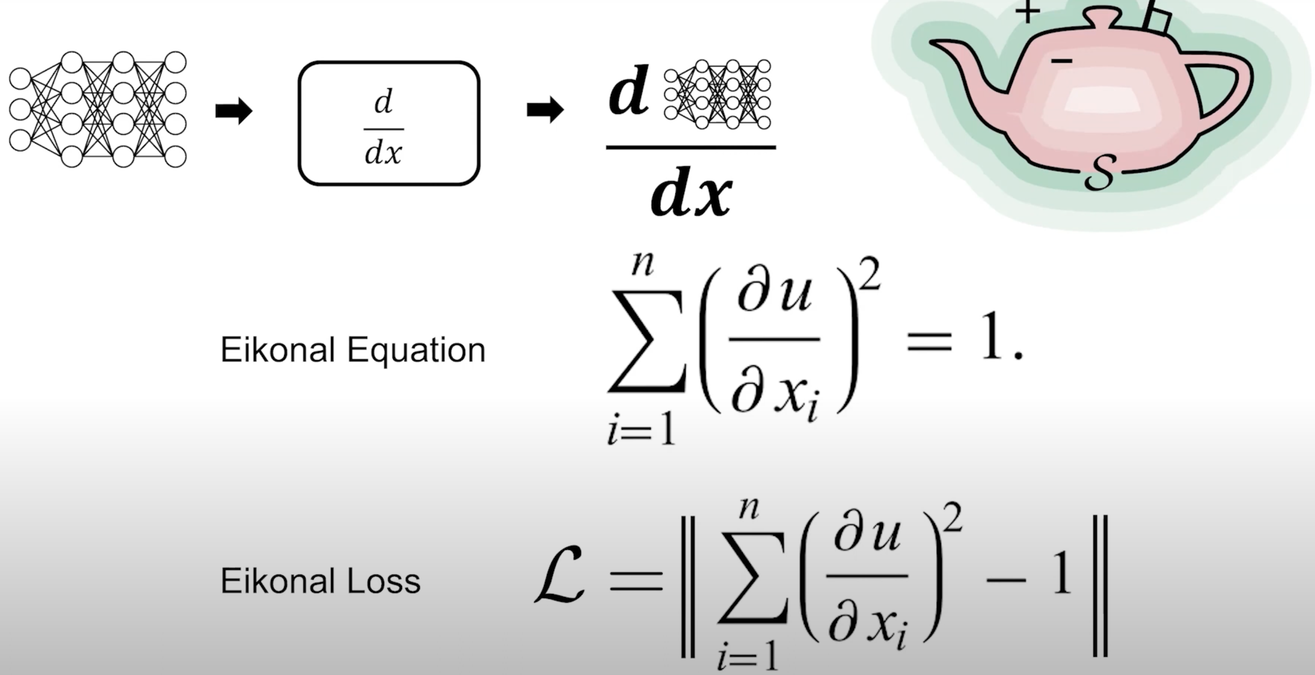
For example the Eikonal equation forces the neural network has a derivative as 1. Adding the eikonal loss then promises the neural network valid.
Generally, this kind of problems are: the solutions are constrained by its partial derivatives.
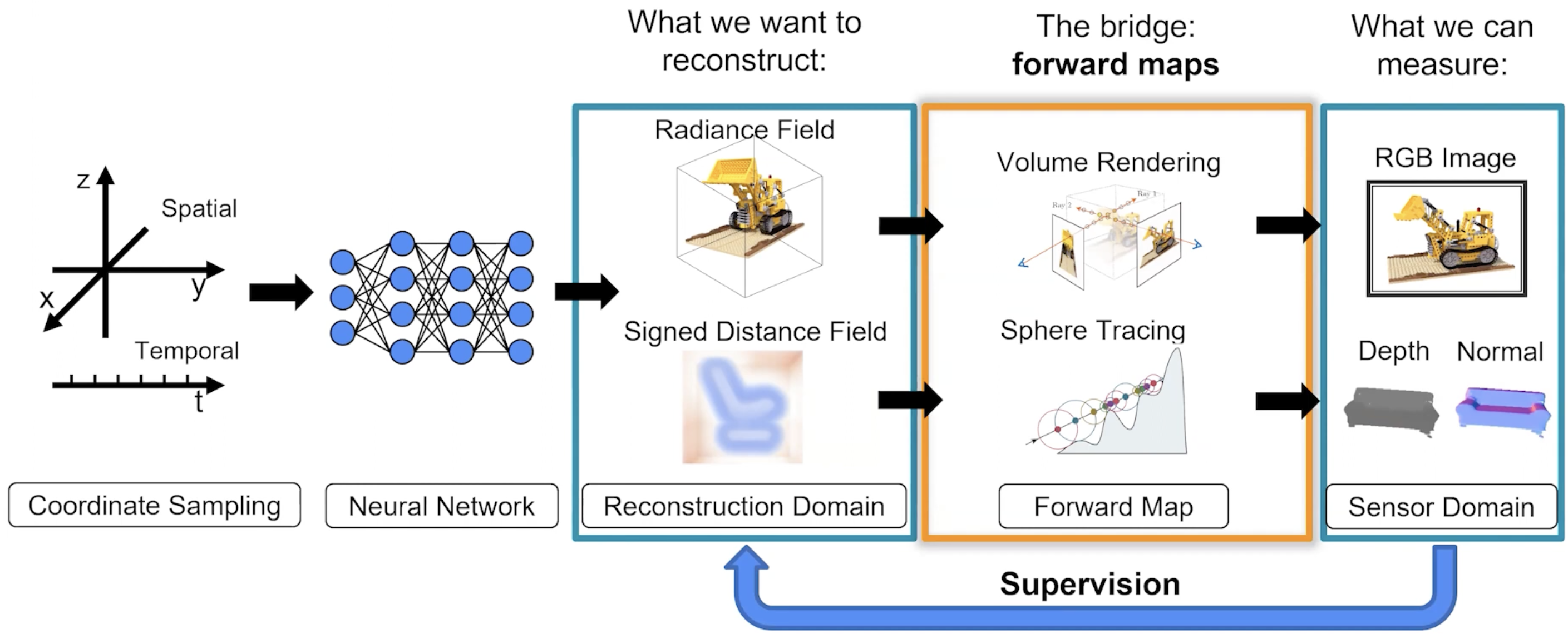
\[\text{Reconstruction} \rightarrow \hat 1()\rightarrow \text{Sensor domain}\\\text{Reconstruction} == \text{Sensor domain}\]
Q&A:
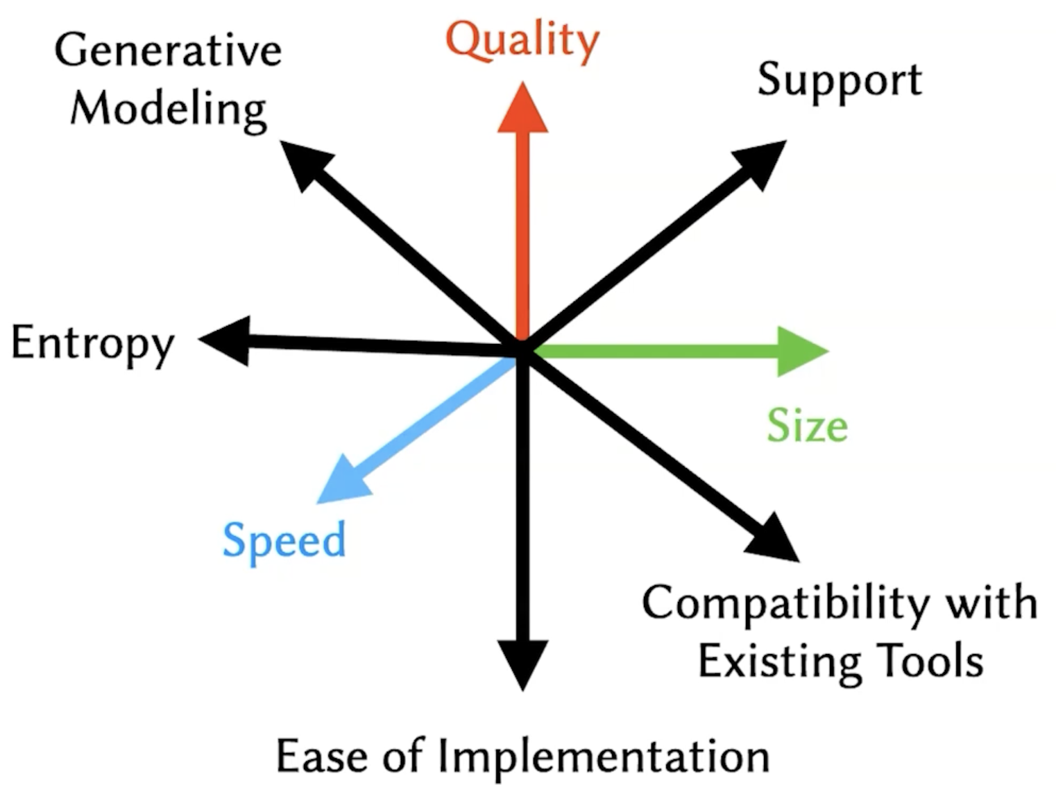
You may choose one proper representation depending on your own application
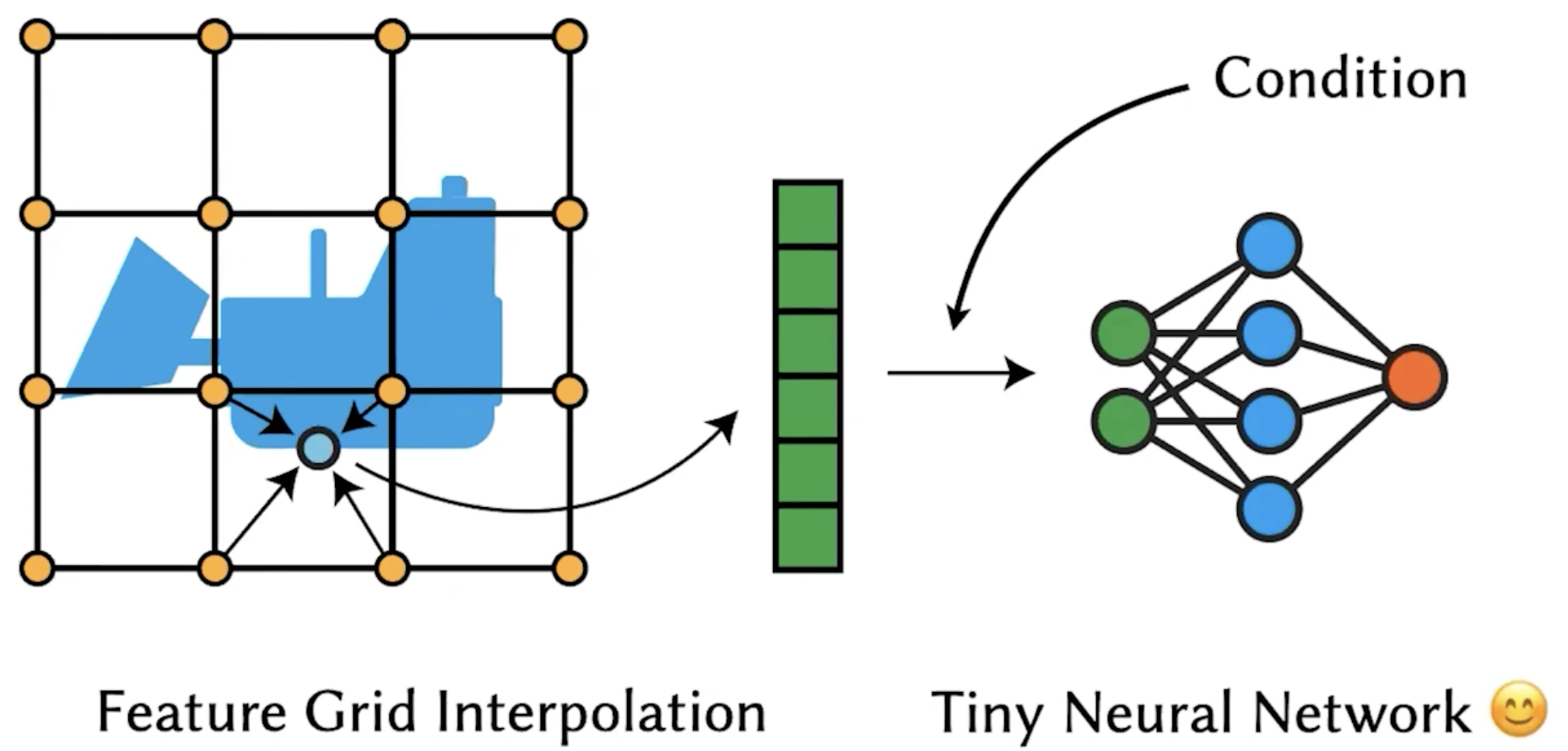
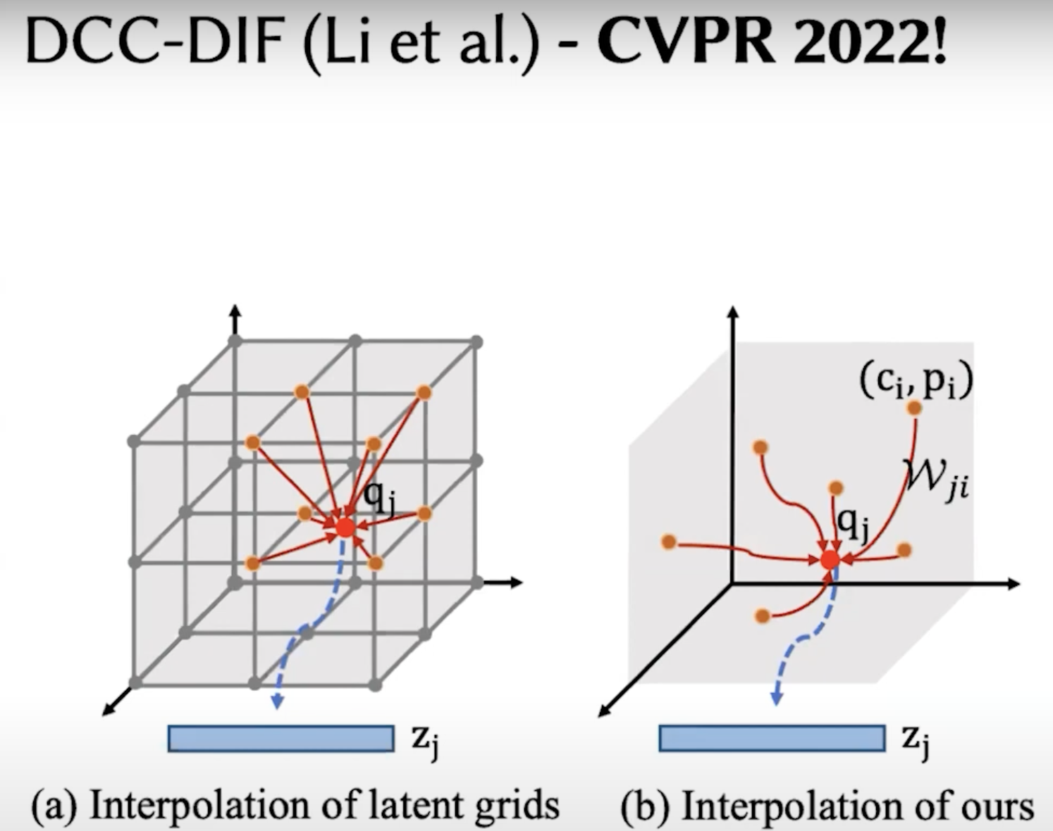
Input is too huge. Then you need too huge neural network. So, this grid interpolation acts like a "position encoding", which encodes the low dimensional features into high dims.
NeRFusion CVPR22: online!
Cons:
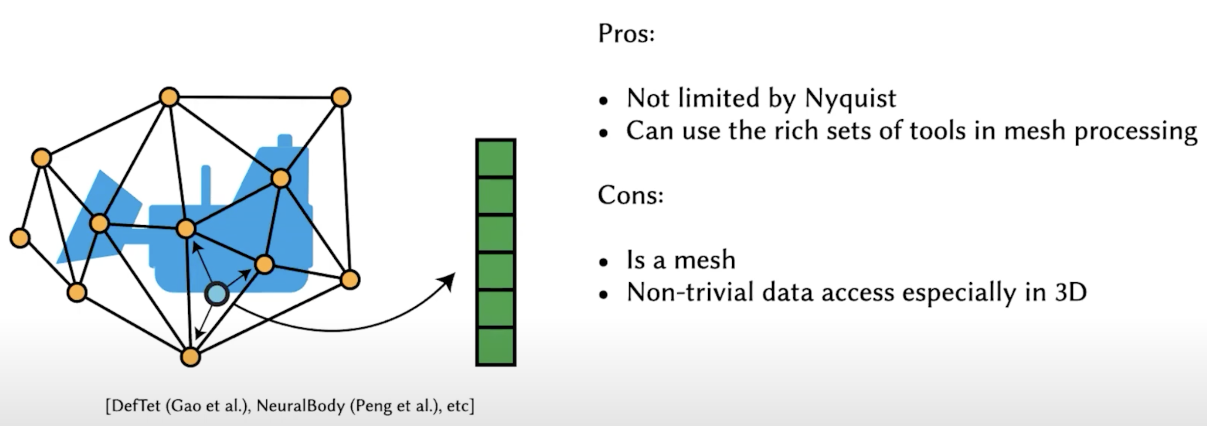
Unstructed grids. Compared with point clouds, meshes have connectivity info.
Something like project a 3D grid into an axis to get levels of planes.
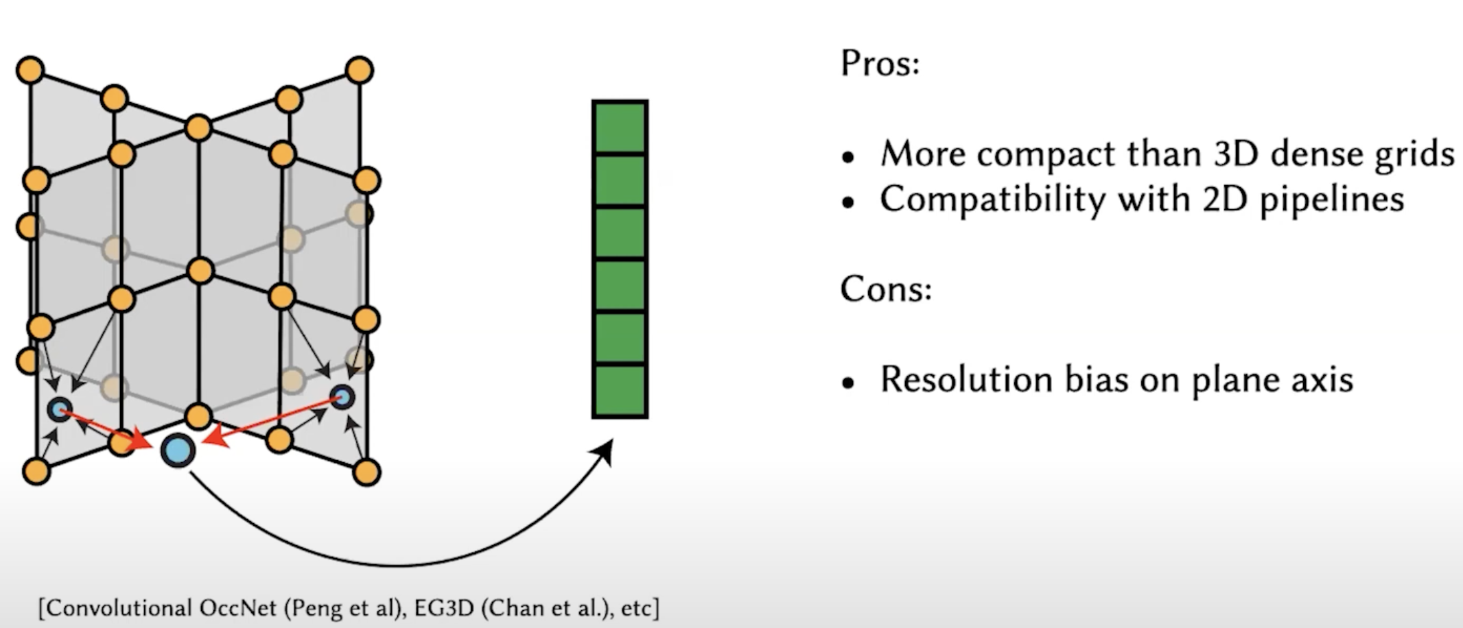
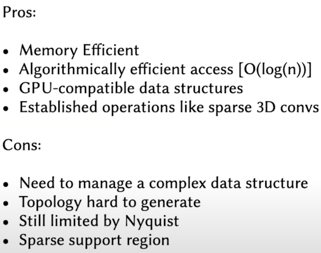
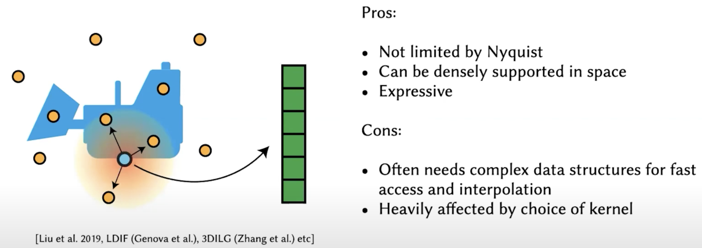
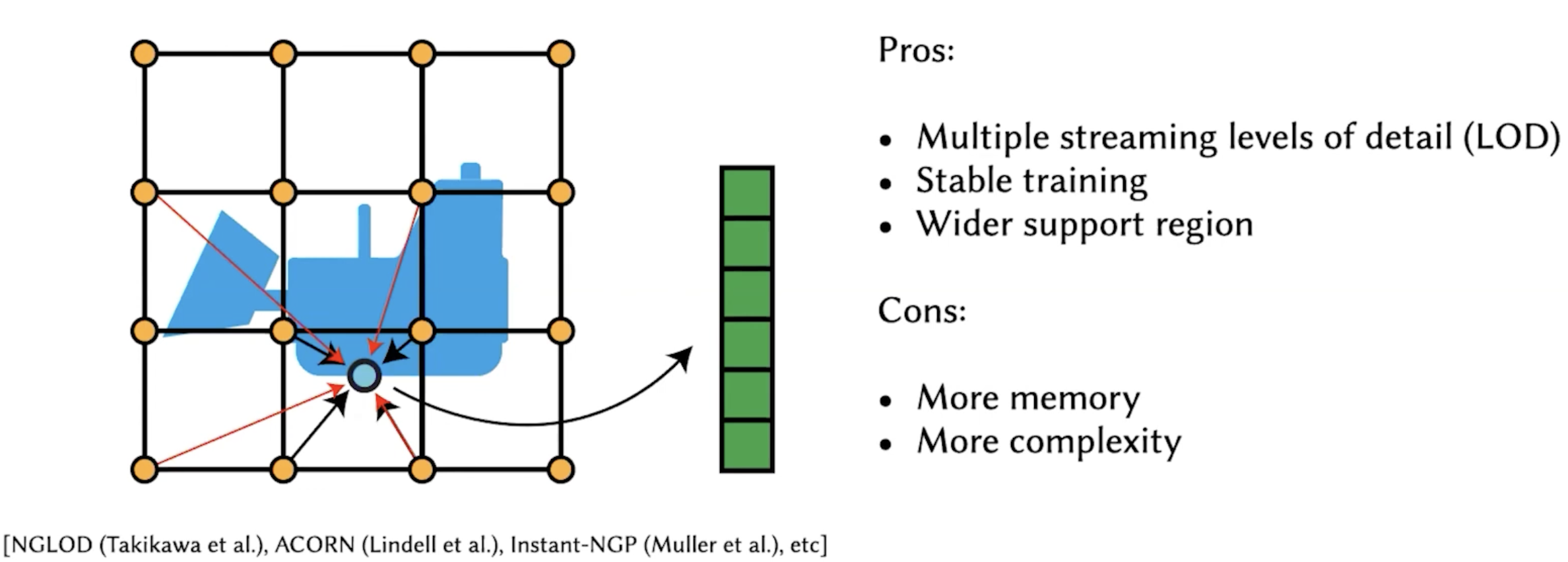
Pros:
Cons:
This is not very wise in my opinion. It is just a temporary tradeoff given nowadays' technologies. Coz everything will be 3D in the future.
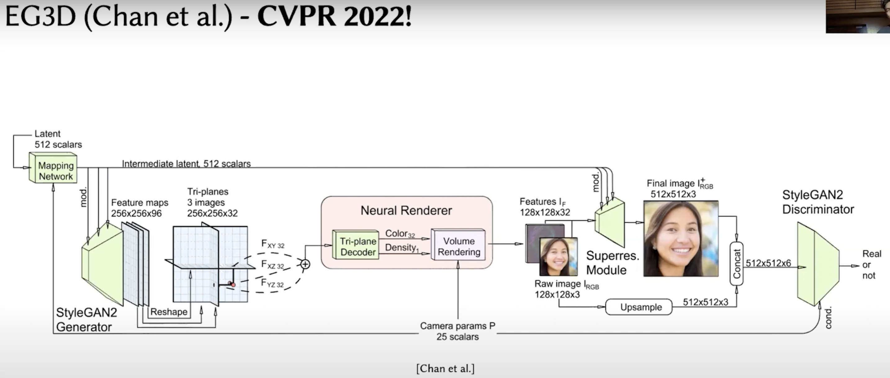 Generate 2D images from different camera views (perhaps). Key point is the tri-plane representation of 3D features.
Pros:
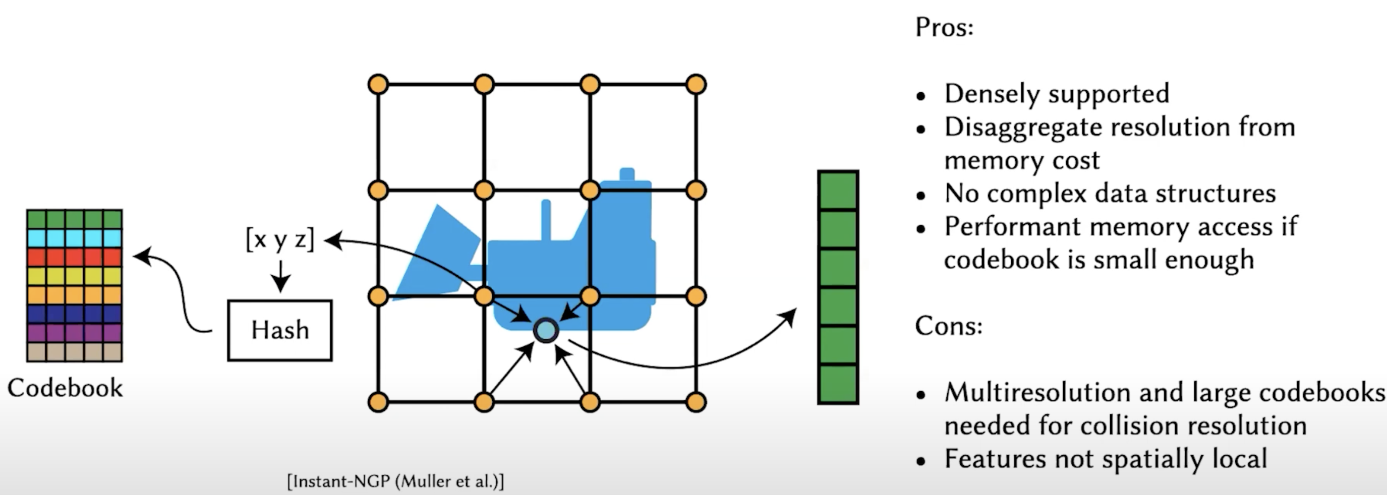 \[[x,y,z]\text{ coordinates}\rightarrow \text{Hash function()} \rightarrow \text{Fixed size codebook}\] Pros:
Cons:
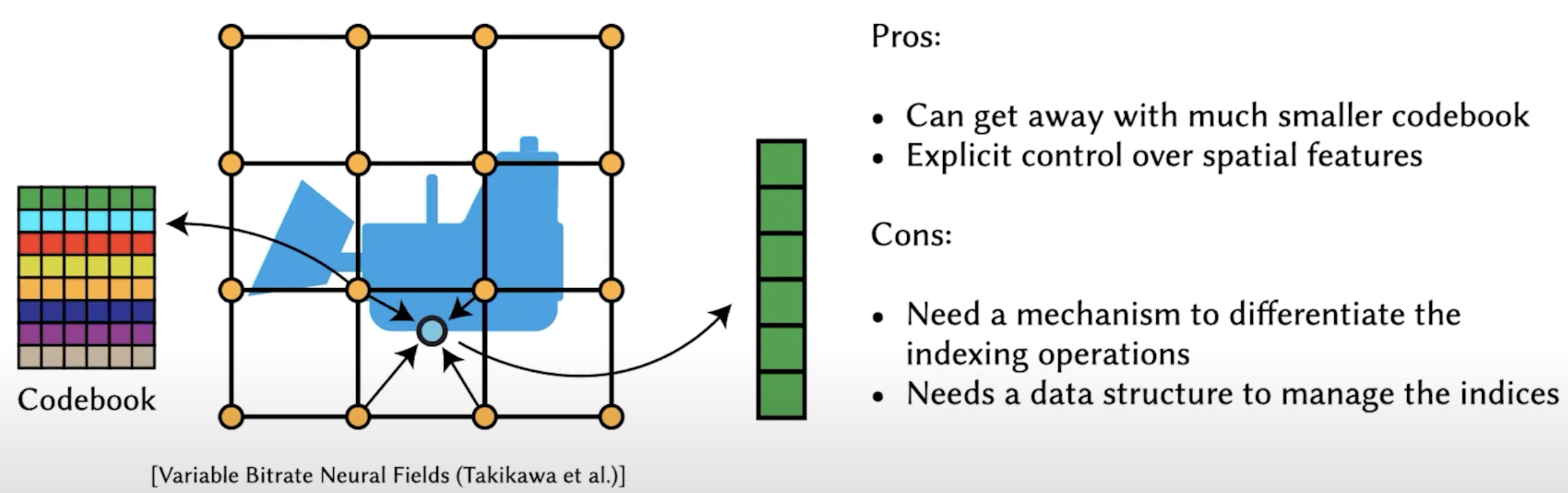
Instead of storing features of points in grids, store a (index to a) code in a codebook. The size of the codebook is fixed, so the overall size can be controlled as much smaller.
cons:
Commonly used method in computer graphics